Joe Report

GITHUB PROJECT LINK – Project2a.ipynb

GITHUB PROJECT LINK – Project2b.ipynb

Exploring Entanglement, BSM, and Teleportation, Project Overview

Project Goals:

• To get hands on experience performing entanglement, BSM (Bell State Measurement), and Teleportation. These will serve as the foundations for further experiments.

Project Outcome:

• You get a chance to see how qubits become entangled through a gate, how entangled qubits are measured, and also how to combine entanglement and qubits to perform teleportation.
• Project 2a: we create qubit superposition, entanglement and BSM results and draw them on a histogram
• Project 2b: we create qubit superposition and entanglement, then introduce network and qubit messengers, as well as BSM to perform teleportation, including a Pauli correction

Tools:

• Python, Qiskit, Jupyter Notebook

Dependencies:

PowerShell-level project dependencies:

• qiskit, qiskit-aer, notebook, matplotlib

Python-level imports:

• qiskit: QuantumCircuit, transpile
• qiskir_aer: AerSimulator
• qiskit.visualization: plot_histogram
• matplotlib.pyplot: plt

Project Setup Guide

Note: You will need to have completed the setup of the tools from Part 1 of the tutorial series for the final virtual environment workspace first before beginning this project. This is necessary in order to have your folders and directories organized, and to make sure you’re already capable of running the necessary tools. Please complete that portion first so you can become familiar with the way everything interacts.

Begin the project by installing the dependencies you will need:

• Open Powershell as the local user
• Verify that you are running python 3.8 or later (current release is 3.14 at the time of this tutorial [Yes, in Python version 3.14 is considered more recent than version 3.8 due to their version naming conventions])
  • Run:
    • python --version
• In PowerShell, navigate to your Qiskit Project Directory you created in Part 1, example:
  • Run:
    • cd C:\Users\[username]\OneDrive\Documents\Python Projects\Qiskit\
• Create a new venv for the project in the Qiskit folder, where you should already have built the virtual environment for the final project and see venv_superposition_ciphertext:
  • Run:
    • python -m venv venv_Project2
    • Your virtual environment for the project has been created
• Activate the venv_Project1 virtual environment:
  • Run:
    • Set-ExecutionPolicy -Scope Process -ExecutionPolicy Bypass
    • This will temporarily bypass script security for this session of PowerShell only
  • Run:
    • .\venv_Project1\Scripts\activate
    • You’ll now see (venv_Project2) before PS in your PowerShell command window, which tells you that your project’s virtual environment is now active.
• Install your PowerShell-level dependencies:
  • Run:
    • pip install qiskit matplotlib
    • pip install notebook
    • pip install qiskit-aer
    • pip install pylatexenc
• Make sure you are in the JupyterNotebooks directory in PS that you created during the first tutorial:
  • Navigate in PowerShell:
    • cd <your chosen project directory path>\JupyterNotebooks\
  • Open Jupyter Notebook from PS while you’re inside the \JupyterNotebooks\ directory, Run:
    • jupyter notebook
• A browser with Jupyter Notebook and a loopback address should appear, with an empty file directory.
• Keep the browser window open for the next steps.

Open Jupyter Notebook

You should already be running Jupyter Notebook from the previous section.

Create your Project 2 Notebooks

• In Jupyter, navigate to:
  • On the righthand, top side of the file list goto:
    • New > Python 3
  • Close the popup window for the ‘Untitled’ notebook
  • Click the Rename Button at the top, change the file name to: Project2a.ipynb
  • Click the Project2a.ipynb file to reopen the project window
  • If it asks you which Kernel to use, make sure you select Python 3.
  • Repeat the steps for Project2b.ipynb

Project Steps Review

Project 2 Part A – Entanglement and BSM

Let the Coding Begin

If you prefer, you can access the GitHub project repository directly and skip the step by step instructions here, but the step by step break down of lines of code is really useful:

Calling All Modules

The only new module we called for in either part of this project was transpile. The other modules already were listed and explained in Project 1.

# Use inline matplotlib for VS Code
%matplotlib inline

from qiskit import QuantumCircuit, transpile
from qiskit_aer import AerSimulator
from qiskit.visualization import plot_histogram
import matplotlib.pyplot as plt

What exactly is happening here?

• We are importing transpile from qiskit to convert high-level quantum circuits into versions that can run efficiently on a specific backend, adapting the gates and qubit layout to the device’s constraints. Aslo optimizes the circuits to reduce depth and redundant operations, improving performance.

Sourcecode Overview: Project2 Part A

This is for Project2a where we entangle two qubits after placing them both into superposition, rotate them and align their bell state and computational basis, then conduct a BSM and analyze the relevant output using histograms

We build our circuit using QuantumCircuit:

# ------------------------------
# 1. Import Dependencies
# ------------------------------
%matplotlib inline

from qiskit import QuantumCircuit, transpile
from qiskit_aer import AerSimulator
from qiskit.visualization import plot_histogram
import matplotlib.pyplot as plt
import networkx as nx

# ------------------------------
# 2. Initialize Quantum Circuit
# ------------------------------
# Two qubits (Q0, Q1) and two classical bits (C0, C1)
qc = QuantumCircuit(2, 2)

# ------------------------------
# 3. Create Entanglement
# ------------------------------
# Hadamard on Q0 to create superposition
qc.h(0)
qc.h(1)
# CNOT to entangle Q0 and Q1
qc.cx(0, 1)

# ------------------------------
# 4. Bell-State Measurement (BSM)
# ------------------------------
# Measure both qubits into classical bits
qc.measure([0, 1], [0, 1])

# ------------------------------
# 5. Execute Circuit and Plot Histogram
# ------------------------------
simulator = AerSimulator()

# Transpile the circuit for the simulator
qc_transpiled = transpile(qc, simulator)

# Run the circuit on the simulator
result = simulator.run(qc_transpiled, shots=1024).result()

# Get counts and plot histogram
counts = result.get_counts()
plot_histogram(counts)
plt.show()

# Map classical outcomes to Bell states
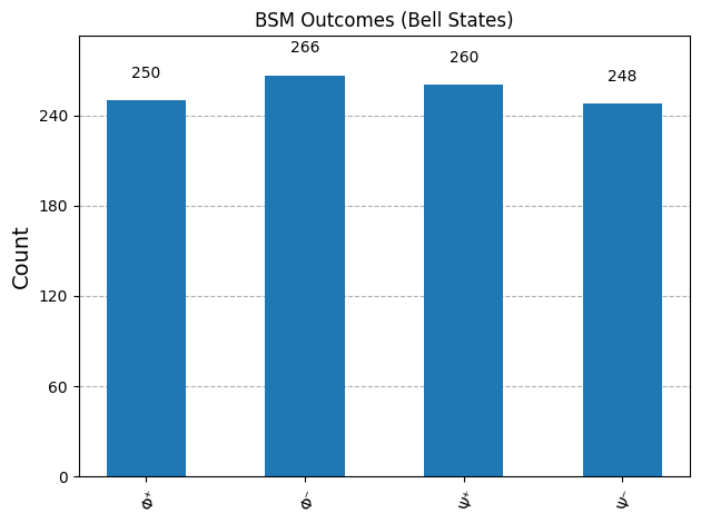
bell_labels = {'00': 'Φ⁺', '01': 'Φ⁻', '10': 'Ψ⁺', '11': 'Ψ⁻'}

# Replace counts keys for plotting
counts_labeled = {bell_labels[k]: v for k, v in counts.items()}

plot_histogram(counts_labeled, title="BSM Outcomes (Bell States)")
plt.show()

What exactly is happening here?

• We initialized a circuit via QuantumCircuit with 2 qubits (Q0, Q1) and 2 classical bits (C0, C1), because we will need these in our circuit to perform entanglement and to hold our post BSM classical values
• We passed qubit 0 and 1 through a Hadamard gate to create superposition
• We used a CNOT gate to entangle both of the qubits (Q0,Q1), creating a new quantum system in a simulated Hilbert space
• We then used the qc.measure() function to calculate the BSM and obtain results
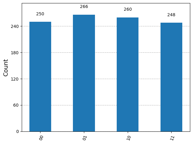
• Next, we posted the results on a histogram to display how Bell States collapse into their four potential states randomly with qubits are in superposition.

Project Output Examples

BSM and Classical outputs after entanglement and subsequent measurement

Project 2 Part B – Entanglement, Messenger, BSM, and Teleportation

Let the Coding Begin

If you prefer, you can access the GitHub project repository directly and skip the step by step instructions here, but the step by step break down of lines of code is really useful:

Calling All Modules

The only new module we called for in either part of this project was transpile. The other modules already were listed and explained in Project 1.

# ==============================
# Project 2 – Part B: Quantum Teleportation
# ==============================

# ------------------------------
# 1. Import Dependencies
# ------------------------------
%matplotlib inline

from qiskit import QuantumCircuit, transpile
from qiskit.visualization import plot_histogram
import matplotlib.pyplot as plt

What exactly is happening here?

• We are importing transpile from qiskit to convert high-level quantum circuits into versions that can run efficiently on a specific backend, adapting the gates and qubit layout to the device’s constraints. Aslo optimizes the circuits to reduce depth and redundant operations, improving performance

Sourcecode Overview: Project2 Part A

For Project 2b, we first put two qubits into superposition and entangle them. A third messenger qubit is introduced and entangled with the pair. Using a Hadamard gate, we align the message and entangled qubits’ Bell and computational bases, then perform a Bell State Measurement (BSM). The resulting classical bits are sent to the receiver qubit, completing the teleportation of the messenger state. Finally, we analyze the outcomes and Pauli corrections with histograms to visualize the process and results

We build our circuit using QuantumCircuit:

# ==============================
# Project 2 – Part B: Quantum Teleportation
# ==============================

# ------------------------------
# 1. Import Dependencies
# ------------------------------
%matplotlib inline

from qiskit import QuantumCircuit, transpile
from qiskit.visualization import plot_histogram
import matplotlib.pyplot as plt

# ------------------------------
# 2. Initialize Quantum Circuit
# ------------------------------
# Q0 = message qubit, Q1/Q2 = entangled pair
# C0/C1 = classical bits for BSM
qc = QuantumCircuit(3, 2)  # 3 qubits, 2 classical bits

# ------------------------------
# 3. Prepare the entangled pair (Q1-Q2)
# ------------------------------
qc.h(1)      # Hadamard on Q1
qc.cx(1, 2)  # CNOT to entangle Q1 and Q2

# ------------------------------
# 4. Bell-State Measurement (BSM) on message + entangled qubit
# ------------------------------
qc.cx(0, 1)  # CNOT: message qubit controls entangled qubit
qc.h(0)      # Hadamard on message qubit
qc.measure([0, 1], [0, 1])  # Measure Q0 + Q1 into C0 + C1

# ------------------------------
# 5. Execute Circuit and Get Counts
# ------------------------------
simulator = AerSimulator()
qc_transpiled = transpile(qc, simulator)
result = simulator.run(qc_transpiled, shots=1024).result()
bsm_counts = result.get_counts()

# ------------------------------
# 6. Map classical outcomes to Bell states
# ------------------------------
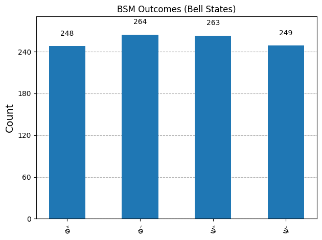
bell_labels = {'00': 'Φ⁺', '01': 'Φ⁻', '10': 'Ψ⁺', '11': 'Ψ⁻'}
bsm_counts_labeled = {bell_labels[k]: v for k, v in bsm_counts.items()}

# Plot BSM outcomes
plot_histogram(bsm_counts_labeled, title="BSM Outcomes (Bell States)")
plt.show()

# ------------------------------
# 7. Map BSM outcomes to Pauli corrections
# ------------------------------
# Classical bits -> Pauli on Q2
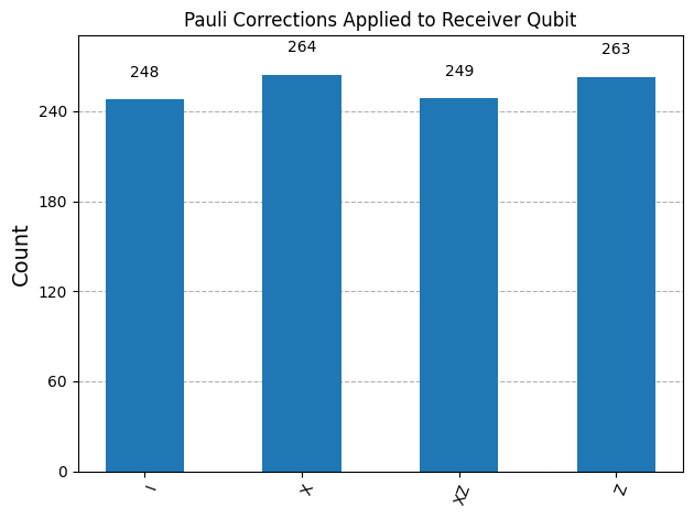
pauli_map = {'00': 'I', '01': 'X', '10': 'Z', '11': 'XZ'}
pauli_counts = {pauli_map[k]: v for k, v in bsm_counts.items()}

# Plot histogram of Pauli corrections
plot_histogram(pauli_counts, title="Pauli Corrections Applied to Receiver Qubit")
plt.show()

What exactly is happening here?

• We initialized a quantum circuit via QuantumCircuit with 3 qubits (Q0, Q1, Q2) and 2 classical bits (C0, C1). Q0 is the message qubit, Q1 and Q2 form the entangled pair, and the classical bits store measurement results for teleportation.
• We applied a Hadamard gate to qubit 1 to create superposition, then a CNOT gate from Q1 to Q2 to entangle them, forming the entangled pair needed for teleportation.
• The messenger qubit (Q0) was entangled with Q1 using a CNOT and then passed through a Hadamard gate to prepare for the Bell State Measurement (BSM).
• We performed a BSM by measuring Q0 and Q1 into classical bits C0 and C1.
• We executed the circuit on a simulator and collected the measurement counts.
• The classical outcomes were mapped to Bell states to show how the entangled qubits collapse into the four possible states, which were displayed on a histogram.
• We also mapped the BSM outcomes to Pauli corrections to indicate what operations would be applied to Q2 to complete the teleportation, visualized in a second histogram.

Project Output Examples

BSM outputs after entanglement

Pauli correction applied on Q2 after Q0 BSM transmitted

Project Conclusions

This project explored how superposition, entanglement, Bell-state measurement, and classical communication work together to form a complete quantum teleportation protocol. By implementing the process step by step in Qiskit and analyzing the resulting measurement statistics with histograms, we were able to observe how quantum states are transferred through correlations rather than physical transmission of information.

Approaching the problem from a systems and architecture perspective makes it clear that teleportation is not a single operation, but a coordinated quantum–classical workflow. The project demonstrates how probabilistic measurement outcomes still lead to reliable state reconstruction through structured correlations and conditional corrections, providing a practical foundation for understanding distributed quantum systems and future quantum networking protocols.

I will go over the process flows and more in-depth in Project 2 Post Project Reflections piece, as well as the many ways we can use this data and additional considerations. After that, we will be delving into different Quantum Algorithms and their functionality in Part 4 of the tutorial.