Joe Report

GITHUB PROJECT LINK – Project1.ipynb

Exploring Qubit Superposition and Measurement, Project Overview

Project Outcome:

• You get a chance to see how qubits behave probabilistically, see how measurement collapses a qubit, and visualize it on a Bloch sphere.

Tools:

• Python, Qiskit, Jupyter Notebook

Dependencies:

PowerShell-level project dependencies:

• qiskit, qiskit-aer, notebooks, matplotlib, ipython, pylatexenc

Python-level imports:

• qiskit: QuantumCircuit
• qiskir_aer: AerSimulator
• qiskit.visualization: plot_bloch_multivector, plot_histogram
• qiskit.quantum_info: Statevector
• matplotlib.pyplot: plt

Project Setup Guide

Note: You will need to have completed the setup of the tools from Part 1 of the tutorial series for the final virtual environment workspace first before beginning this project. This is necessary in order to have your folders and directories organized, and to make sure you’re already capable of running the necessary tools. Please complete that portion first so you can become familiar with the way everything interacts.

Begin the project by installing the dependencies you will need:

• Open Powershell as the local user
• Verify that you are running python 3.8 or later (current release is 3.14 at the time of this tutorial [Yes, in Python version 3.14 is considered more recent than version 3.8 due to their version naming conventions])
  • Run:
    • python --version
• In PowerShell, navigate to your Qiskit Project Directory you created in Part 1, example:
  • Run:
    • cd C:\Users\[username]\OneDrive\Documents\Python Projects\Qiskit\
• Create a new venv for the project in the Qiskit folder, where you should already have built the virtual environment for the final project and see venv_superposition_ciphertext:
  • Run:
    • python -m venv venv_Project1
    • Your virtual environment for the project has been created
• Activate the venv_Project1 virtual environment:
  • Run:
    • Set-ExecutionPolicy -Scope Process -ExecutionPolicy Bypass
    • This will temporarily bypass script security for this session of PowerShell only
  • Run:
    • .\venv_Project1\Scripts\activate
    • You’ll now see (venv_Project1) before PS in your PowerShell command window, which tells you that your project’s virtual environment is now active.
• Install your PowerShell-level dependencies:
  • Run:
    • pip install qiskit matplotlib notebook
    • pip install qiskit-aer
    • pip install pylatexenc
    • pip install ipython
• Make sure you are in the JupyterNotebooks directory in PS that you created during the first tutorial:
  • Navigate in PowerShell:
    • cd <your chosen project directory path>\JupyterNotebooks\
  • Open Jupyter Notebook from PS while you’re inside the \JupyterNotebooks\ directory, Run:
    • jupyter notebook
• A browser with Jupyter Notebook and a loopback address should appear, with an empty file directory.
• Keep the browser window open for the next steps.

**** How exciting! If you’ve made it this far, then you’re ready to begin working on quantum projects! Congratulations! Let’s continue with how to get started in Jupyter Notebook.****

Working in Jupyter Notebook

You should already be running Jupyter Notebook from the previous section.

Create your first Notebook

• In Jupyter, navigate to:
  • On the righthand, top side of the file list goto:
    • New > Python 3
  • Close the popup window for the ‘Untitled’ notebook
  • Click the Rename Button at the top, change the file name to: Project1.ipynb
  • Click the Project1.ipynb file to reopen the project window
  • If it asks you which Kernel to use, make sure you select Python 3.

Let the Coding Begin

We’re going to first import our QisKit modules. You can go through this step by step if you want to understand how everything is working.

If you prefer, you can access the GitHub project repository directly and skip the step by step instructions here, but the step by step break down of lines of code is really useful:

Calling All Modules

Here we will walk through the project code line by line, with an extended explanation of what is happening:

# Use inline matplotlib for VS Code
%matplotlib inline

from qiskit import QuantumCircuit
from qiskit_aer import AerSimulator
from qiskit.visualization import plot_histogram, plot_bloch_multivector
from qiskit.quantum_info import Statevector
import matplotlib.pyplot as plt

• %matplotlib inline is telling Python to display the results directly in the notebook or editor.
• QuantumCircuit is the class for building quantum circuits, and this is where you define qubits, classical bits, and gate operations.
• AerSimulator is a simulator backend that lets you run circuits locally in simulation.
• plot_histogram and plot_bloch_multivector are visualization tools, histogram showing distribution of measurement outcomes and block_multivector showing a Bloch sphere to help visualize how quantum bits work in superposition.
• Statevector allows us to cheat and view the quantum state of the circuit without collapsing the bit. This let’s us calculate how probabilities and amplitudes impact the circuit, as well as determining the impact of using certain gates.
• matplotlib.pyplot is a Python plotting library used to display plots that works with visualization functions.

Building the Circuit

Next, we will build our circuit using QuantumCircuit:

qc = QuantumCircuit(1, 1)
qc.h(0)
qc.measure(0, 0)

What exactly is happening here?

• QuantumCircuit(1, 1) creates a quantum circuit with 1 quibit and 1 classical bit
• qc.h(0) applies a Hadamard gate to qubit 0, putting the qubit into superposition with a 50/50 chance of measuring as a 0 or 1
• qc.measure(0,0) measures qubit 0 and then stores the result in classical bit 0

Overview: We create qubit and classical bit holders, apply a hadamard gate to place the qubit into superposition, and then measure the bit, effectively collapsing the superposition state and turning it into a classical bit (1 or 0)

Drawing the Circuit and Simulation

Ok, let’s draw our circuit image and then simulate ‘shots’, or iterations of the circuit from start to finish, then plot the outcomes:

# Draw circuit (static image)
qc.draw('mpl')

# Run QASM simulator
qasm_sim = AerSimulator()
qasm_result = qasm_sim.run(qc, shots=1024).result()
counts = qasm_result.get_counts()
print("Measurement counts:", counts)

# Plot histogram
plot_histogram(counts)
plt.show()

What exactly is happening here?

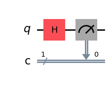
• qc.draw(‘mpl’) draws a static diagram of the circuit using matplotlib and shows qubits, classical bits, and gates cleary. ‘mpl’ renders it as an inline image in Jupyter.
• Aer_Simulator() sets up a QASM simulator backend to model real quantum measurement and produces classical outputs
• qasm_sim.run(qc, shots=1024).result() runs the circuit 1024 times (shots) for the sample measurement and retrieves the results
• qasm_result.get_counts() counts the number of time the bit returned as a 0 or 1
• print(counts) displays the measurement results
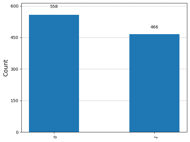
• plot_histogram(counts) creates a bar chart showing the frequency of 0 or 1 outcomes after measurement.
• plt.show() displays histogram plot inline in Jupyter.

Overview: We first draw a diagram of the circuit (Image 1) to display in Jupyter, then run a quantum simulator repeatedly to observe trends in measurement outcomes and demonstrate how amplitude probabilities work when applying a gate. Finally, we visualize the results in a histogram (Image 2) to show the distribution of classical bits after measurement.

Creating the Bloch Sphere

Finally, we are going to create our Bloch Sphere to visualize how the qubit looks when suspended between states:

qc_sv = QuantumCircuit(1)
qc_sv.h(0)

statevector = Statevector.from_instruction(qc_sv)

# Plot Bloch sphere as a static figure
fig = plot_bloch_multivector(statevector, figsize=(6,6))
plt.show()

What exactly is happening here?

• QuantumCircuit(1) this creates a new circuit with 1 qubit and no classical bit, separate from the one we made earlier, specifically for the Bloch Sphere
• qc_sv.h(0) we apply the Hadamard gate again, placing the qubit in superposition, but we aren’t measuring this time – just plotting
• Statevector.from_instruction(qc_sv) queries the state of the qubit while in superposition without causing collapse to a classical bit
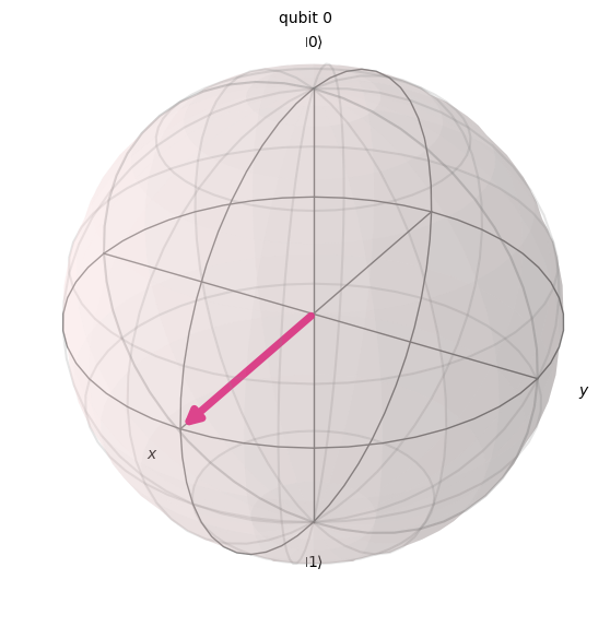
• plot_bloch_multivector(statevector, figsize=(6,6))
  plt.show() plots the qubit state on a sphere, to show where it exists while in superposition, between 0 and 1, and displays it inline within Jupyter

Overview: We create a new, single qubit, quantum circuit, but this time we don’t want to measure it, we just want to view it’s position without collapsing it. So we pass the qubit through a Hadamard gate again, but this time we use Statevector to view it’s state and correlate that state onto a Bloch Sphere to demonstrate superposition visually.

Sourcecode Overview

# Use inline matplotlib
%matplotlib inline

from qiskit import QuantumCircuit
from qiskit_aer import AerSimulator
from qiskit.visualization import plot_histogram, plot_bloch_multivector
from qiskit.quantum_info import Statevector
import matplotlib.pyplot as plt

# ----------------------------
# 1. Circuit with measurement
# ----------------------------
qc = QuantumCircuit(1, 1)
qc.h(0)
qc.measure(0, 0)

# Draw circuit (static image)
qc.draw('mpl')

# Run QASM simulator
qasm_sim = AerSimulator()
qasm_result = qasm_sim.run(qc, shots=1024).result()
counts = qasm_result.get_counts()
print("Measurement counts:", counts)

# Plot histogram
plot_histogram(counts)
plt.show()

# ----------------------------
# 2. Bloch sphere circuit
# ----------------------------
qc_sv = QuantumCircuit(1)
qc_sv.h(0)

statevector = Statevector.from_instruction(qc_sv)

# Plot Bloch sphere as a static figure
fig = plot_bloch_multivector(statevector, figsize=(6,6))
plt.show()

Project Output Examples

Measurement counts: {‘0’: 558, ‘1’: 466}

First Quantum Circuit visualization:

Histogram results:

Bloch Sphere results, where the north and south poles represent 0 and bit classical bits, and the area between them represents the superposition of the qubit when viewed with Statevector:

Conclusion

You now have a foundational understanding of the tools needed to run quantum simulations. More importantly, you should be starting to grasp the underlying concepts and seeing how they relate to real world quantum computing.

That concludes our first hands-on project. Hopefully, this exercise has helped you learn both the practical and conceptual aspects of quantum computing, giving you a foundation to start applying that knowledge.

Our next tutorial section will focus on the importance of quantum gates, exploring how they function and what they’re used for, beyond the introductory Hadamard gate.